Defining velocity models
Using the Velocity Model form (prepare > Seismic > Domain Conversion > Velocity Model) you can define any number of velocity models based on time horizons and - for the apparent velocities method – also on depth markers.
A velocity model definition comprises at least one zone with a time horizon at its base. For each zone, you need to specify the velocity profile to use. The interval velocity can be entered as a constant, a function (see Velocity types – Methods of defining velocity profiles) or can be calculated from the time horizon in combination with markers (if you have them). A constant interval velocity is used for the domain conversion of objects deeper than the deepest zone.
To create a velocity model definition
- Open the Velocity Model form (prepare > Seismic > Domain Conversion).
- From the Model drop-down list, select 'Create new' and type the name for a new velocity model. Then click the plus sign (
 ) to create the model and activate the controls on the form.
 - In the Source drop-down list, select the folder that contains the time horizons you want to use to create the velocity model. Only sources which contain time horizons are available for selection.
- Marker set (Only applicable for velocity model based on markers.) Select the marker set that contains the markers to be used for the velocity model.
- In the Base Surface column, select the base surface for a velocity layer. The drop-down list contains all the available time horizons in 2D grid format within your selected 'Source'.
- Click in the Velocity Type column to select the velocity type for each zone. Velocity type is the method by which the velocity profile within a zone is generated. Choose from a number of options, some of which have unique functionality. For details on these options, see Velocity types – Methods of defining velocity profiles.
- If you selected any of the V0k velocity types, or 'Vint from user input', specify the layer velocity in the V [m/s] column:
- If you selected 'Vint from user input', enter the value for Vint in the table cell. Vint is constant for the layer.
- If you selected Vint, Vinst or Vavg per V0k method, enter the value for V0 in the table cell. Alternatively, you can select a laterally varying V0, see 'Using laterally varying V0 and k' below.
- If you selected a V0k velocity type, specify the velocity gradient ‘k’ (acceleration factor/compaction factor) in the K column.
- To use a constant k-gradient, type it into the table cell (higher values mean larger velocity increase).
- Alternatively, you an select a laterally varying k-gradient stored as a k property, see 'Using laterally varying V0 and k' below.
- If you selected Velocity Type 'Vavg = Water Velocity Profile Avg', enter a factor between -1 and 1 in the column Vwater Profile Factor. The application makes use of three lookup tables for water velocity; Vmin for low water velocity, Vavg for average water velocity and Vmax for high water velocity (lookup factors '-1', '0' and '1' respectively). Based on the value you enter, the table values are weighted. For example, when you enter 0.5, the average of the values of Vavg and Vmax will be taken. For the lookup values, see Velocity types – Methods of defining velocity profiles.
- In the Function Reference column, select a reference function. It defines the reference for the velocity function in the selected layer. V0 of each layer corresponds to the selected reference time. Function reference can be a constant or a 2D grid with time values available in your selected source. A typical choice for function reference is ‘seabed’ or 0 (project datum).
- In case you selected a marker set, the last column of the table shows the marker symbol (
 ) if a marker for the selected base surface is present in the selected marker set.
 - In the Underburden entry field at the base of the form, enter the Vint value for the constant interval velocity to be used for domain conversion of objects deeper than the deepest zone.
- On the Well Velocity Interpolation tab, select the type of interpolation that determines how average velocities calculated from horizon time and top depth are interpolated between the sparse well control points. You can choose between the following interpolation methods:
- Inverse Distance Weighting (IDW) This uses the distance-weighted algorithm to interpolate the time horizon using the marker locations as constraining input. Enter the power value (between 0 and 6). The Power is the exponent used for the weighting of the distances.
- Ordinary Kriging (legacy) This method does not make use of the industry standard Kriging library and is performance optimized. Choose the function and enter the values for Major Range, Minor Range and Azimuth(GN).
- Variogram type - Exponential, Exponential Power (the power value sets the lateral extension of the Kriging), Gaussian or Spherical.
- Major range - Specify the distance at which the values become independent (the variogram reaches its plateau). The distance is measured in the direction with the greatest spatial continuity.
- Minor range - Specify the distance at which the values become independent (the variogram reaches its plateau). The distance is measured in the direction with the least spatial continuity and is orthogonal to the major direction.
- Azimuth(GN) - Enter the azimuth (angle with Northing direction) of the axis corresponding with the major range.
- Click Apply or OK to finalize your velocity model that you can use in domain conversion.
Model tab
Using laterally varying V0 and k
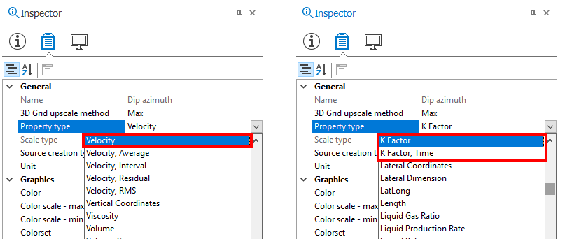
For V0k velocity functions, you can incorporate a laterally varying V0 and k-gradient in your function. To do this, you have to have V0 and k as a property available for the time horizon of interest. For V0, the property needs to be of type 'Velocity'; for k the property needs to be of type 'K-Factor' or 'K-Factor, time' (depending on the function you use), which you can set in the Property Inspector  . Once you have these properties, you can select them in the V [m/s] and K columns on the Velocity Model form for them to be used in the function. Note that the property must be defined at each node of the time horizon 2D grid.
Well Velocity Interpolation tab (only for 'Vint from marker depth')
Velocity model objects can be exported and imported into other solutions.